Synthetic covariance matrices

Synthetic covariance matrices for seismic arrays.

This module provides functions to generate theoretical and estimated synthetic covariance matrices from analytical models. These are useful for validating array processing methods, exploring the relationship between wavefield physics and covariance matrix structure, and for producing reference covariances to compare against observed data.

The station geometry is described by a list of Stats objects with assigned geographical coordinates. All spatial calculations delegate to station_local_coordinates() and pairwise_distance_matrix_from_stats() from the covseisnet.spatial module.

Functions

• plane_wave_field() — monochromatic plane-wave field at each station.

• plane_wave_covariance() — rank-1 covariance matrix of a monochromatic plane wave.

• surface_noise_covariance() — theoretical isotropic 2D (surface-wave) noise covariance via the Bessel function \(J_0\).

• volume_noise_covariance() — theoretical isotropic 3D (body-wave) noise covariance via the sinc function.

• spherical_wave_field() — monochromatic spherical wave field from a point source.

• spherical_wave_covariance() — rank-1 covariance matrix of a monochromatic spherical wave.

• random_noise_covariance() — covariance matrix estimated from independent Gaussian noise snapshots.

covseisnet.synthetic.plane_wave_field(stats: list[Stats], frequency: float, slowness: float, azimuth: float) → ndarray

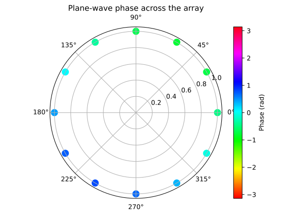
Monochromatic plane-wave field at each station.

Computes the complex wavefield \(\psi_i\) of a monochromatic plane wave propagating in a homogeneous medium with apparent slowness \(s_0\) and frequency \(f\), recorded at station \(i\) located at local east-north coordinates \((x_i, y_i)\):

\[\psi_i = \exp\!\left(-\imath\, k \bigl(\sin\theta\, x_i + \cos\theta\, y_i\bigr)\right)\]

where \(k = 2\pi f s_0\) is the apparent wavenumber (rad/km), and \(\theta\) is the propagation azimuth measured clockwise from north. The local coordinates are computed with a flat-Earth projection (see station_local_coordinates()).

Parameters:

• stats (list of Stats) -- Stats objects of the network stations. Each must have a coordinates attribute with longitude and latitude keys.

• frequency (float) -- Wave frequency in hertz.

• slowness (float) -- Apparent slowness in seconds per kilometre (s/km).

• azimuth (float) -- Propagation direction measured clockwise from north in degrees.

Returns:

numpy.ndarray -- Complex array of shape (n_stations,) with the wavefield amplitude and phase at each station.

See also

plane_wave_covariance()

Example

import numpy as np
import matplotlib.pyplot as plt

import covseisnet as csn
from covseisnet.synthetic import plane_wave_field

# Build a circular array of 12 stations
n = 12
angles = np.linspace(0, 2 * np.pi, n, endpoint=False)
lons = 0.5 * np.cos(angles) / 111.195 + 2.0
lats = 0.5 * np.sin(angles) / 111.195 + 48.0
stats = [
    csn.NetworkStream.read()[0].stats.__class__()
    for _ in range(n)
]
for i, s in enumerate(stats):
    s.coordinates = {"longitude": lons[i], "latitude": lats[i],
                     "elevation": 0.0}

wavefield = plane_wave_field(stats, frequency=1.0, slowness=0.3,
                             azimuth=45.0)
fig, ax = plt.subplots(subplot_kw={"projection": "polar"})
sc = ax.scatter(angles, np.abs(wavefield), c=np.angle(wavefield),
                cmap="hsv", vmin=-np.pi, vmax=np.pi, s=100)
plt.colorbar(sc, label="Phase (rad)")
ax.set_title("Plane-wave phase across the array")

covseisnet.synthetic.plane_wave_covariance(stats: list[Stats], frequency: float, slowness: float, azimuth: float) → CovarianceMatrix

Rank-1 covariance matrix of a monochromatic plane wave.

Computes the outer product of the plane-wave field \(\boldsymbol{\psi}\) (see plane_wave_field()):

\[C_{ij} = \psi_i\, \psi_j^*\]

The resulting matrix is Hermitian, positive semi-definite, and has rank 1, meaning its eigenvalue spectrum consists of a single non-zero eigenvalue equal to \(N\) (the number of stations) and \(N-1\) zero eigenvalues.

Parameters:

• stats (list of Stats) -- Stats objects of the network stations.

• frequency (float) -- Wave frequency in hertz.

• slowness (float) -- Apparent slowness in seconds per kilometre (s/km).

• azimuth (float) -- Propagation direction measured clockwise from north in degrees.

Returns:

CovarianceMatrix -- Hermitian covariance matrix of shape (n_stations, n_stations).

See also

plane_wave_field(), spherical_wave_covariance()

covseisnet.synthetic.surface_noise_covariance(stats: list[Stats], frequency: float, slowness: float) → CovarianceMatrix

Theoretical covariance matrix for isotropic 2D (surface-wave) noise.

Under the assumption of isotropic surface-wave noise distributed uniformly around the array, the cross-spectral density between stations \(i\) and \(j\) separated by a distance \(d_{ij}\) is given by the zero-order Bessel function of the first kind (Lobkis and Weaver, 2001):

\[C_{ij}(f) = J_0\!\left(k\, d_{ij}\right)\]

where \(k = 2\pi f s_0\) is the wavenumber. The diagonal entries equal 1 (since \(J_0(0) = 1\)). The matrix is real, symmetric, and Toeplitz (for a linear array). This is the theoretical limit reached by averaging sufficiently many independent plane-wave snapshots distributed uniformly in azimuth.

Parameters:

• stats (list of Stats) -- Stats objects of the network stations. Each must have a coordinates attribute with longitude, latitude, and elevation keys.

• frequency (float) -- Wave frequency in hertz.

• slowness (float) -- Apparent slowness in seconds per kilometre (s/km).

Returns:

CovarianceMatrix -- Real-valued (promoted to complex) Hermitian covariance matrix of shape (n_stations, n_stations).

See also

volume_noise_covariance()

covseisnet.synthetic.volume_noise_covariance(stats: list[Stats], frequency: float, slowness: float) → CovarianceMatrix

Theoretical covariance matrix for isotropic 3D (body-wave) noise.

Under the assumption of uniformly distributed isotropic noise sources in three dimensions (body-wave diffuse field), the cross-spectral density between two receivers separated by distance \(d_{ij}\) is (Weaver and Lobkis, 2001):

\[C_{ij}(f) = \frac{\sin(k\, d_{ij})}{k\, d_{ij}}\]

where \(k = 2\pi f s_0\) is the wavenumber. This is the unnormalised sinc function. The diagonal entries equal 1 in the limit \(d_{ij} \to 0\).

Note

NumPy's numpy.sinc() uses the normalised convention \(\operatorname{sinc}(x) = \sin(\pi x)/(\pi x)\). The physical sinc \(\sin(kd)/(kd)\) is therefore evaluated as numpy.sinc(k * d / numpy.pi).

Parameters:

• stats (list of Stats) -- Stats objects of the network stations. Each must have a coordinates attribute with longitude, latitude, and elevation keys.

• frequency (float) -- Wave frequency in hertz.

• slowness (float) -- Apparent slowness in seconds per kilometre (s/km).

Returns:

CovarianceMatrix -- Real-valued (promoted to complex) Hermitian covariance matrix of shape (n_stations, n_stations).

See also

surface_noise_covariance()

covseisnet.synthetic.spherical_wave_field(stats: list[Stats], frequency: float, slowness: float, source: tuple[float, float, float]) → ndarray

Monochromatic spherical wave field from a point source.

Computes the wavefield \(\psi_i\) of an outgoing monochromatic spherical wave emitted by a point source at source and recorded at each station \(i\):

\[\psi_i = \frac{1}{r_i + \varepsilon} \exp\!\left(-\imath\, k\, r_i\right)\]

where \(r_i\) is the straight-ray distance (km) between the source and station \(i\), \(k = 2\pi f s_0\) the wavenumber, and \(\varepsilon = 10^{-6}\) km a regularisation constant that avoids division by zero for a station co-located with the source.

Parameters:

• stats (list of Stats) -- Stats objects of the network stations. Each must have a coordinates attribute with longitude, latitude, and elevation keys.

• frequency (float) -- Wave frequency in hertz.

• slowness (float) -- Apparent slowness in seconds per kilometre (s/km).

• source (tuple of float) -- Source position as (longitude, latitude, depth) where longitude and latitude are in decimal degrees and depth is in kilometres (positive downward below sea level).

Returns:

numpy.ndarray -- Complex array of shape (n_stations,) with the wavefield amplitude and phase at each station.

See also

spherical_wave_covariance(), plane_wave_field()

covseisnet.synthetic.spherical_wave_covariance(stats: list[Stats], frequency: float, slowness: float, source: tuple[float, float, float]) → CovarianceMatrix

Rank-1 covariance matrix of a monochromatic spherical wave.

Computes the outer product of the spherical-wave field \(\boldsymbol{\psi}\) (see spherical_wave_field()):

\[C_{ij} = \psi_i\, \psi_j^* = \frac{\exp\!\bigl(-\imath\, k\,(r_i - r_j)\bigr)} {(r_i + \varepsilon)(r_j + \varepsilon)}\]

Like the plane-wave covariance, this matrix is Hermitian, positive semi-definite, and has rank 1. Unlike the plane-wave case, the amplitude of each off-diagonal entry decreases with the distance from the source, reflecting geometrical spreading. This model is useful for testing source-localisation algorithms.

Parameters:

• stats (list of Stats) -- Stats objects of the network stations.

• frequency (float) -- Wave frequency in hertz.

• slowness (float) -- Apparent slowness in seconds per kilometre (s/km).

• source (tuple of float) -- Source position as (longitude, latitude, depth) where longitude and latitude are in decimal degrees and depth is in kilometres (positive downward below sea level).

Returns:

CovarianceMatrix -- Hermitian covariance matrix of shape (n_stations, n_stations).

See also

spherical_wave_field(), plane_wave_covariance()

covseisnet.synthetic.random_noise_covariance(stats: list[Stats], n_snapshots: int = 100, seed: int | None = None) → CovarianceMatrix

Covariance matrix of spatially uncorrelated Gaussian noise.

Estimates the covariance matrix of white (spatially uncorrelated) noise by averaging \(M\) outer products of independent random snapshots:

\[\hat{\mathbf{C}} = \frac{1}{M}\sum_{m=1}^{M} \boldsymbol{n}_m\, \boldsymbol{n}_m^{\dagger}\]

where each snapshot \(\boldsymbol{n}_m \in \mathbb{C}^N\) is drawn from a standard complex normal distribution (independent standard normals for real and imaginary parts). In expectation, \(\mathbb{E}[\hat{\mathbf{C}}] = \mathbf{I}_N\), and the result converges to the identity matrix as \(M \to \infty\). This model corresponds to a fully incoherent field with maximum coherence spectral width \(\sigma = 1\).

Parameters:

• stats (list of Stats) -- Stats objects of the network stations. Only the number of stations \(N = \texttt{len(stats)}\) is used.

• n_snapshots (int, optional) -- Number of independent snapshots \(M\) to average. Larger values yield a result closer to \(\mathbf{I}_N\). Defaults to 100.

• seed (int or None, optional) -- Seed for the random number generator. Pass an integer for reproducible results. Defaults to None (non-deterministic).

Returns:

CovarianceMatrix -- Complex Hermitian covariance matrix of shape (n_stations, n_stations).