Time normalization

This example shows how to perform a temporal normalization of traces with different methods. These methods are described in the paper from Bensen et al. (2007), and a ubiquitous in ambient noise seismology to mitigate the effect of localized seismic sources that may bias the analysis of cross-correlation functions.

import matplotlib.pyplot as plt

import covseisnet as csn

Read waveforms

This section reads an example stream of seismic data shipped with Obspy. The stream contains three traces, which are highpass at a very high frequency to see more details in the synchronization.

# Read the example stream. Using the read method without arguments reads the
# example stream shipped with Obspy.
stream = csn.read()

# Highpass filter the stream for a better illustration
stream.filter("highpass", freq=1)

# Print the stream
print(stream)

3 Trace(s) in NetworkStream (synced):
BW.RJOB..EHZ | 2009-08-24T00:20:03.000000Z - 2009-08-24T00:20:32.990000Z | 100.0 Hz, 3000 samples
BW.RJOB..EHN | 2009-08-24T00:20:03.000000Z - 2009-08-24T00:20:32.990000Z | 100.0 Hz, 3000 samples
BW.RJOB..EHE | 2009-08-24T00:20:03.000000Z - 2009-08-24T00:20:32.990000Z | 100.0 Hz, 3000 samples

Normalization methods

We here show the trace normalized with different methods, namely a one-bit normalization, and a smooth envelope removal technique. The methods are applied to the stream, and the normalized traces are stored in a list. Considering the seismic trace \(x(t)\) the normalized trace \(\hat x(t)\) is obtained with

\[\hat x(t) = \frac{x(t)}{Ax(t) + \epsilon}\]

where \(A\) is an function or operator applied to the trace \(x(t)\), and \(\epsilon > 0\) is a regularization value to avoid division by 0. The application \(A\) is defined by the method parameter. We distinguish two cases:

• If method = "onebit", the operator \(A\) is the modulus operation with \(Ax = |x|\), and therefore

  \[\hat x(t) = \frac{x(t)}{|x(t)| + \epsilon} \approx \text{sign}(x(t))\]

  In this case, the method calls the covseisnet.signal.modulus_division.

• If the method="smooth", the operator \(A\) is defined as a Savitzky-Golay filter applied to the Hilbert envelope of the trace. The Savitzky-Golay filter is defined by the smooth_length and smooth_order parameters.

# Initialize the list of normalized streams
normalization_methods = ["onebit", "smooth"]
normalized_streams = []

# Normalize the stream with the different methods
for method in normalization_methods:
    normalized_stream = stream.copy()
    normalized_stream.time_normalize(method=method)
    normalized_streams.append(normalized_stream)

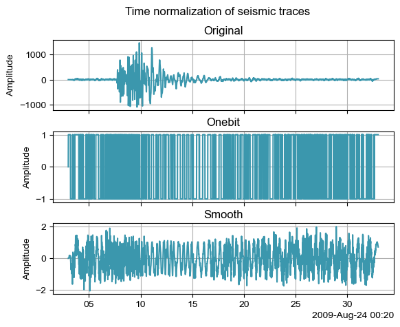
Comparison

This section compares the original stream with the normalized streams. The traces are plotted in a figure, where the original stream is plotted first, and the normalized streams are plotted below.

# Concatenate the original stream with the normalized streams
streams = [stream] + normalized_streams
labels = ["original"] + normalization_methods

# Create gigure
fig, axes = plt.subplots(len(streams), sharex=True, gridspec_kw={"hspace": 0.3})

# Plot each case
for ax, stream, label in zip(axes, streams, labels):
    ax.plot(stream.times("matplotlib"), stream.traces[0].data)
    ax.set_title(label.title())
    ax.set_ylabel("Amplitude")
    ax.grid()

# Set the title
fig.suptitle("Time normalization of seismic traces")

# Set the x-axis label
csn.plot.dateticks(axes[-1])