Cross-correlation

This example shows how to calculate the cross-correlation functions from five sensors of the USArray network stacked over two months from January 1, 2006 to March 1, 2006. At first, we made sure to access the example USArray data and inventory. If for any reason, the data is not available under the data folder under the docs/sources directory of the repository, or if you would like to run this script outside of the repository, the data will be automatically downloaded with the covseisnet.data.download_usarray_data function (see in the second cell of this notebook).

Note that the sampling rate of these traces is voluntarily low to reduce the size of the example data and the speed of the calculations. The data is downsampled at 0.2 Hz.

import matplotlib.pyplot as plt

import covseisnet as csn

Read and pre-process stream

We first read the example stream and pre-process it. At first, we simply detrend and high-pass filter the data. Because the USArray data is not synchronized at these stations, especially in 2006, we synchronize the stream using the method :meth:~covseisnet.stream.NetworkStream.synchronize. This method is automatic and can be used in a custom way. We then normalize the traces for cross-correlation in the time domain.

# Path to the example stream
FILEPATH_WAVEFORMS = "../data/usarray.mseed"
FILEPATH_INVENTORY = "../data/usarray.xml"

# Read example stream
stream = csn.read(FILEPATH_WAVEFORMS)

# Pre-process stream
stream.detrend("linear")
stream.filter("highpass", freq=0.001)
stream.synchronize()
stream.time_normalize(method="smooth", smooth_length=101)

Assign coordinates to the stream

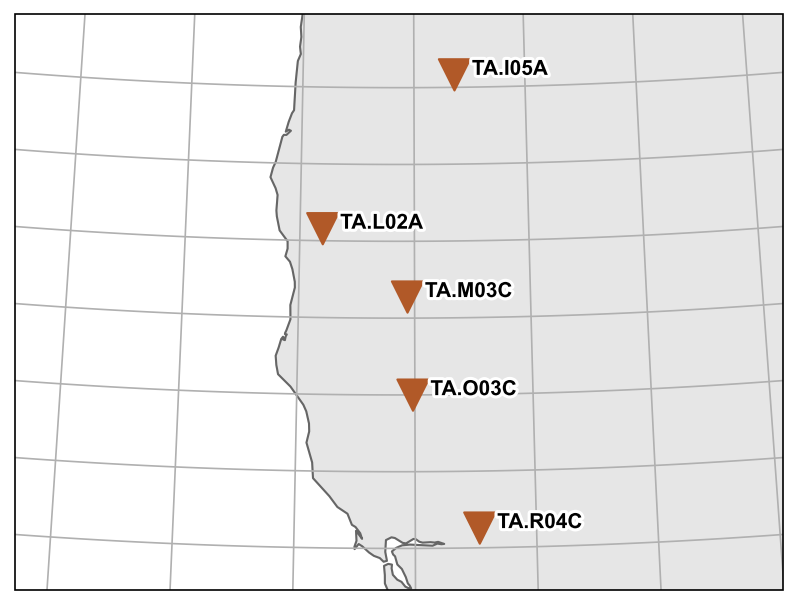
We finally assign the coordinates to the stream using the method :meth:~covseisnet.stream.NetworkStream.assign_coordinates. This method requires the path to the inventory file of the network. If you do not have the inventory file, you can download it with the method :func:~covseisnet.stream.NetworkStream.download_coordinates. These methods deal directly with the :class:~obspy.core.inventory.Inventory object of the traces within the stream. Thanks to a lot of useful methods therein, we can easily plot the inventory on a map and perform other selection tasks.

# Assign coordinates to the stream
stream.assign_coordinates(FILEPATH_INVENTORY)

# Plot inventory
fig = stream.inventory.plot(projection="local", resolution="i")

Covariance matrix

The covariance matrix is calculated using the method covseisnet.covariance.calculate_covariance_matrix. The method returns the times, frequencies, and covariances of the covariance matrix. Among the parameters of the method, the window duration and the number of windows are important to consider. The window duration is the length of the Fourier estimation window in seconds, and the number of windows is the number of windows to average to estimate the covariance matrix.

We can then visualize the covariance matrix at a given time and frequency, and its corresponding eigenvalues.

# Calculate covariance matrix
times, frequencies, covariances = csn.calculate_covariance_matrix(
    stream, window_duration=800, average=500, whiten="window"
)

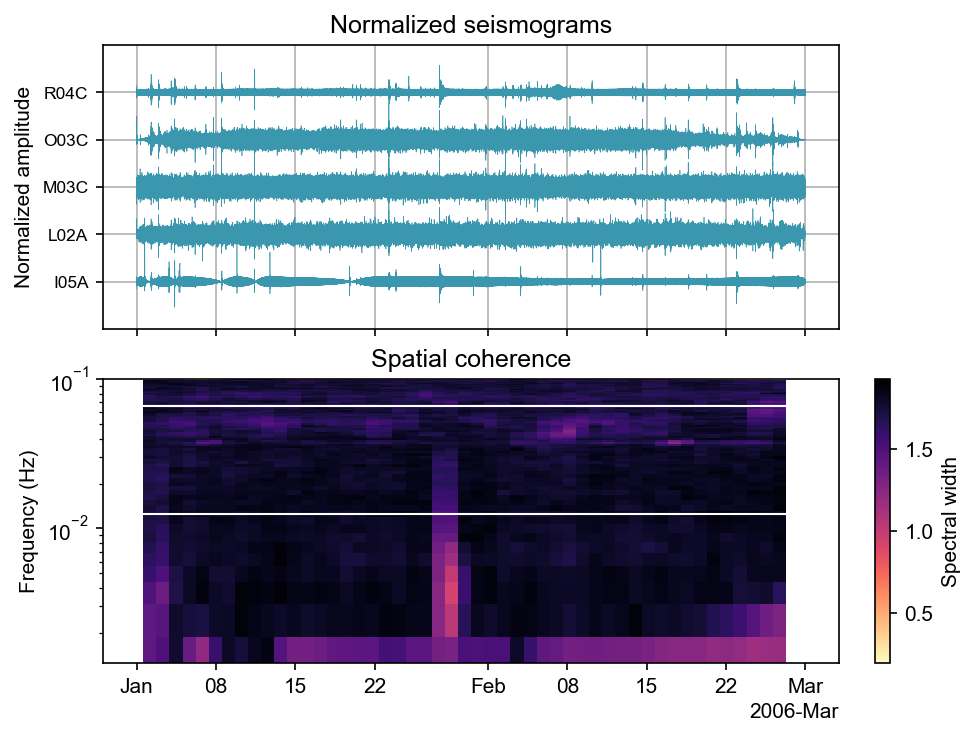
Spectral width

We here extract the coherence from the covariance matrix. The coherence is calculated using the method covseisnet.covariance.CovarianceMatrix.coherence. It can either measure the spectral width of the eigenvalue distribution at each frequency, or with applying the formula of the Neumann entropy.

frequency_band = 1 / 80, 1 / 15

# Calculate coherence
coherence = covariances.coherence(kind="spectral_width")

# Show
fig, ax = csn.plot.stream_and_coherence(
    stream, times, frequencies, coherence, trace_factor=0.1
)

# Indicate frequency band
ax[1].axhspan(*frequency_band, facecolor="none", edgecolor="w", clip_on=False)

<matplotlib.patches.Polygon at 0x16757cd70>

Cross-correlation

The cross-correlation matrix is calculated using the method covseisnet.correlation.calculate_cross_correlation_matrix. The method returns the lags, pairs names, and cross-correlation functions calculated from the inverse Fourier transform of the covariance matrix. The method requires the covariance matrix as input.

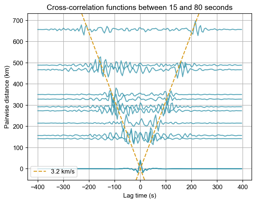
We can then visualize the cross-correlation functions between the sensors as a function of the lag time and the distance between the sensors. Since we selected a frequency band where no clear localized source is observed in the covariance matrix spectral width, we can assume that the cross-correlation functions are symmetric as we observe in the plot. We indicate the speed of Rayleigh waves at 3.2 km/s with dashed lines.

# Calculate cross-correlation
lags, pairs, cross_correlation = csn.calculate_cross_correlation_matrix(
    covariances
)

# Get inter-station distance
distances = csn.pairwise_great_circle_distances_from_stats(
    cross_correlation.stats
)

# Bandpass filter
cross_correlation = cross_correlation.mean(axis=1)
cross_correlation = cross_correlation.bandpass(frequency_band)
cross_correlation = cross_correlation.taper()

# Plot
fig, ax = plt.subplots()
for i_pair, pair in enumerate(pairs):
    cc = cross_correlation[i_pair] / abs(cross_correlation[i_pair]).max() * 40
    ax.plot(lags, cc + distances[i_pair], color="C0", alpha=0.8)

# Plot some velocity
v = 3.2
ax.axline((0, 0), slope=v, color="C1", label=f"{v} km/s", ls="--")
ax.axline((0, 0), slope=-v, color="C1", ls="--")

ax.legend(loc="lower left")
ax.grid()
periods = list(sorted(int(1 / f) for f in frequency_band))
ax.set_title(
    f"Cross-correlation functions between {periods[0]} and {periods[1]} seconds"
)
ax.set_xlabel("Lag time (s)")
ax.set_ylabel("Pairwise distance (km)")

Text(0, 0.5, 'Pairwise distance (km)')