Constant differential times#
This example shows how to calculate the differential travel times of seismic waves in a constant velocity model between two receivers. We first define the model and the sources and receivers coordinates. We then calculate the travel times for each receiver using the class covseisnet.travel_times.TravelTimes, and we calculate the differential travel times using the class covseisnet.travel_times.DifferentialTravelTimes. Finally, we plot the differential travel times on a map.
[1]:
import covseisnet as csn
Create a constant velocity model#
We first create a constant velocity model with a velocity of 5 km/s. In order to do so, we simply need to define the geographical extent of the model, the resolution of the grid, and the velocity.
[2]:
model = csn.velocity.VelocityModel(
    extent=(40, 41, 50, 51, 0, 20),
    shape=(20, 20, 20),
    velocity=3.5,
)
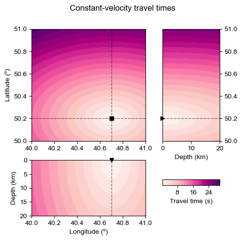
Calculate the travel times between the sources and the receiver#
Each grid point of the model is considered as a source and the receiver is defined by the user. In the example below, the receiver is located at coordinates (40.7, 50.2, 0), somewhere in the model’s domain. The travel times are calculated using the class covseisnet.travel_times.TravelTimes.
We can then represent the travel times on a map using the method covseisnet.plot.grid3d.
[16]:
# Calculate the travel times
travel_time_1 = csn.calculate_travel_times(
    model, receiver_coordinates=(40.7, 50.2, 0)
)

travel_time_2 = csn.calculate_travel_times(
    model, receiver_coordinates=(40.2, 50.9, 0)
)

# Plot the traveltime grid
fig, ax = csn.plot.grid3d(
    travel_time_1, cmap="RdPu", label="Travel time (s)", vmin=0
)

fig.suptitle("Constant-velocity travel times")
[16]:
Text(0.5, 0.98, 'Constant-velocity travel times')
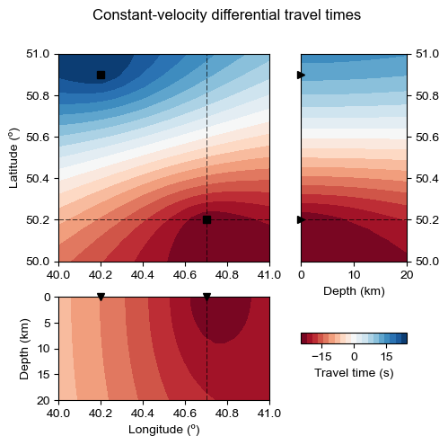
Differential travel times#
The differential travel times are calculated using the class covseisnet.travel_times.DifferentialTravelTimes. The differential travel times are calculated between the two receivers defined above, and shown on a map using the function covseisnet.plot.grid3d.
[29]:
# Calculate the differential travel times
differential_traveltime = travel_time_1 - travel_time_2

# Plot the differential traveltime grid
fig, ax = csn.plot.grid3d(differential_traveltime, label="Travel time (s)")

# Title
fig.suptitle("Constant-velocity differential travel times");