2. Coherence#
[1]:
from pathlib import Path
from pickle import dump

import covseisnet as csn
Read seismograms#
[2]:
# Read
stream = csn.read("../data/undervolc.mseed")
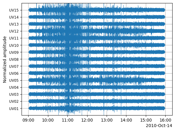
# Pre-process
stream.normalize(global_max=True)
stream.filter("highpass", freq=0.5)
stream.time_normalize(method="smooth", smooth_length=1001)
stream.taper(max_percentage=0.01)
stream.assign_coordinates("../data/undervolc.xml")
# Plot stream
csn.plot.plot_stream(stream, trace_factor=0.1, lw=0.3)
[2]:
<Axes: ylabel='Normalized amplitude'>
Calculate covariance matrix#
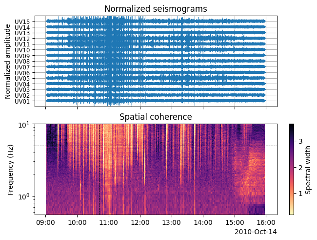
Estimate the covariance matrix by averaging noisy covariance matrices calculated in average=20 50%-overlapping, short window_duration=20-sec windows.
[3]:
# Calculate covariance matrix
times, frequencies, covariances = csn.calculate_covariance_matrix(
    stream, window_duration=20, average=20, whiten="slice"
)

# Save
with open("../data/undervolc_covariance.pickle", "wb") as file:
    dump({"covariances": covariances, "frequencies": frequencies, "times": times}, file)
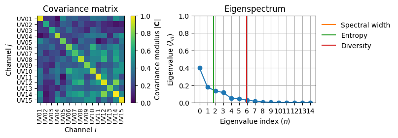
[6]:
# Show covariance from sample window and frequency
t_index = 60
f_index = 100
fig, ax = csn.plot.covariance_matrix_modulus_and_spectrum(covariances[t_index, f_index])
Coherence#
We quantify the spatial coherence of the seismic wavefield by characterizing the distribution of eigenvalues using the spectral width (kind="spectral_width") or the entropy (kind="entropy"). Since the covariance matrix is defined in the frequency domain, we have one value of spectral width or entropy at every frequency and, consequently, the spatial coherence is expressed in time and frequency.
[7]:
# Calculate coherence
coherence = covariances.coherence(kind="spectral_width")

# Show
fig, ax = csn.plot.stream_and_coherence(
    stream,
    times,
    frequencies,
    coherence,
    f_min=0.5,
)

# Mark extracted time and frequency
ax[1].axvline(times[t_index], color="k", linestyle="--", lw=0.7)
ax[1].axhline(frequencies[f_index], color="k", linestyle="--", lw=0.7)
[7]:
<matplotlib.lines.Line2D at 0x740d2ed827b0>