4. Travel times

This first notebook allows to download all necessary data and metadata for the tutorial. This allows the user to get ready with their own data in order to later use the tutorial to analyze their own data.

Note that this tutorial uses Path objects to handle file paths. This is a very convenient way to handle file paths in Python. If you are not familiar with Path objects, you can read the official ``pathlib` documentation <https://docs.python.org/3/library/pathlib.html>`__. Also note that the velocity model is stored as a h5 file, which is a binary file format but not mandatory and implies the use of the h5py library. If you are not familiar with h5 files, you can read the h5py documentation.

from pathlib import Path

import h5py as h5
import numpy as np
import obspy

import covseisnet as csn

Read the velocity model of the Piton de la Fournaise volcano

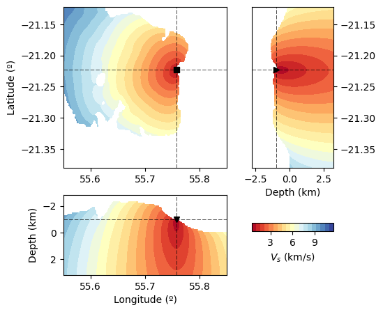
We use the 3D velocity model of the Piton de la Fournaise volcano (Morder et al. 2014), accessible in the supplementary material. We first turn the grid into a h5 file and read it here before filling a regular 3D grid. The model can be displyaed with the grid3d function of the covseisnet.plot function.

Mordret, A., Rivet, D., Landès, M., & Shapiro, N. M. (2015). Three‐dimensional shear velocity anisotropic model of Piton de la Fournaise Volcano (La Réunion Island) from ambient seismic noise. Journal of Geophysical Research: Solid Earth, 120(1), 406-427.

# Read the model
filepath_model = Path("../data/undervolc_vs_mordret_2015.h5").absolute()
velocity_field_name = "Vs"

# The h5 file contains the velocity model in a 3D grid with the following
# dimensions in order: longitude, latitude, depth. The depth and velocity are
# in meters and meters per second, respectively.
with h5.File(filepath_model, "r") as velocity_model:

    # Coordinates
    lon = np.array(velocity_model["longitude"])
    lat = np.array(velocity_model["latitude"])
    depth = np.array(velocity_model["depth"])

    # Velocity
    velocity = np.array(velocity_model[velocity_field_name])

# Get extent
model = csn.velocity.model_from_grid(lon, lat, depth, velocity)

# Plot the grid
fig, ax = csn.plot.grid3d(model, profile_coordinates=[55.7, -21.25, 1], cmap="RdYlBu", label="$V_s$ (km/s)")

stream = csn.read("../data/undervolc.mseed")
stream.assign_coordinates("../data/undervolc.xml")
longitudes = [tr.stats.coordinates.longitude for tr in stream]
latitudes = [tr.stats.coordinates.latitude for tr in stream]
depths = [-tr.stats.coordinates.elevation * 1e-3 for tr in stream]
travel_times = csn.travel_times.TravelTimes(model, receiver_coordinates=(longitudes[2], latitudes[2], depths[2]))
print(travel_times)

travel_times[np.isinf(travel_times)] = np.nan
print(travel_times)

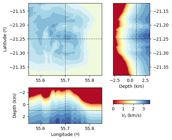
fig, ax = csn.plot.grid3d(
    travel_times,
    receiver_coordinates=(longitudes[2], latitudes[2], depths[2]),
    cmap="RdYlBu",
    label="$V_s$ (km/s)",
)

Using Pykonal to calculate travel times.

/home/eric/WORK/software/covseisnet/covseisnet/travel_times.py:224: RuntimeWarning: divide by zero encountered in scalar divide
  solver.solve()

TravelTimes(
        lon: [55.55, 55.85] with 151 points
        lat: [-21.38, -21.12] with 130 points
        depth: [-2.80, 3.20] with 61 points
        mesh: 1,197,430 points
        nan values: 0 points
        min: 0.432
        max: inf
)
TravelTimes(
        lon: [55.55, 55.85] with 151 points
        lat: [-21.38, -21.12] with 130 points
        depth: [-2.80, 3.20] with 61 points
        mesh: 1,197,430 points
        nan values: 372,659 points
        min: 0.432
        max: 11.604
)