
Matched-field processing#
Matched-field processing on a geographical grid.
This module provides the MatchedFieldProcessing class, which
evaluates the Bartlett matched-field processor (MFP) power over a
GeographicalGrid using pre-computed travel times
and a CovarianceMatrix as input.
The Bartlett MFP is the three-dimensional generalisation of beamforming: the steering vector is now the replica field of a spherical wave rather than a plane wave, so the processor can resolve source depth as well as horizontal position.
The MVDR matched-field processor (Capon) and MUSIC are planned for future releases.
Classes#
MatchedFieldProcessing— Bartlett MFP power on a geographical grid.
- class covseisnet.matchedfield.MatchedFieldProcessing(travel_times: dict[str, TravelTimes])[source]#
Bases:
GeographicalGridBartlett matched-field processing power on a geographical grid.
Given a
CovarianceMatrix\(\mathbf{C} \in \mathbb{C}^{N \times N}\) and a replica vector\[\mathbf{w}(\mathbf{r}, f) = \exp\!\bigl(-2\pi i f \boldsymbol{t}( \mathbf{r})\bigr)\]where \(\boldsymbol{t}(\mathbf{r})\) is the vector of travel times from grid point \(\mathbf{r}\) to every receiver, the Bartlett MFP power is
\[P_{\mathrm{Bartlett}}(\mathbf{r}, f) = \mathbf{w}^\dagger \mathbf{C} \mathbf{w} \;/\; N^2\]where \(N\) is the number of stations.
The result is stored as a 3-D array of shape
(n_lon, n_lat, n_depth)that inherits fromGeographicalGrid.The MVDR processor minimises output power subject to a distortionless constraint on the replica:
\[P_{\mathrm{MVDR}}(\mathbf{r}, f) = \frac{1}{\mathbf{w}^\dagger \mathbf{C}^{-1} \mathbf{w}}\]Note
Planned extensions
MUSIC pseudo-spectrum: projects replica vectors onto the noise subspace of the covariance matrix; offers higher resolution than Bartlett for well-separated sources.
- Parameters:
travel_times (
dict[str,TravelTimes]) -- Dictionary mapping station identifiers to their travel-time grids. All grids must share the same geographical extent and shape.
- travel_times#
The input travel-time grids.
- Type:
dict[str,TravelTimes]
Example
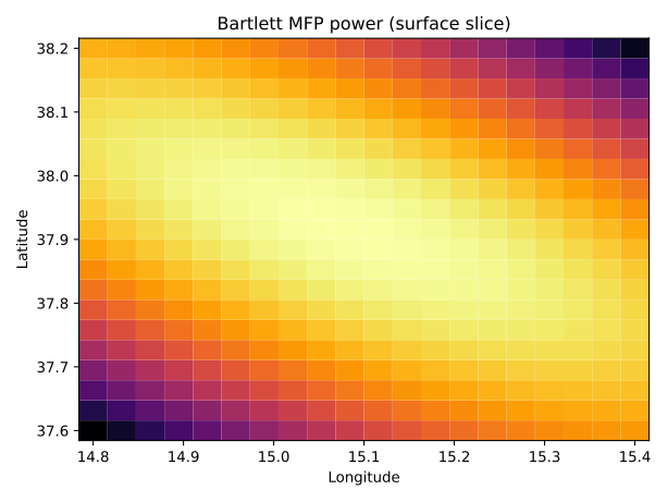
Compute the MFP power for a synthetic spherical wave:
import numpy as np
import matplotlib.pyplot as plt

import covseisnet as csn
from covseisnet.matchedfield import MatchedFieldProcessing
from covseisnet.synthetic import spherical_wave_covariance

stream = csn.read("docs/source/data/undervolc.mseed")
stream.assign_coordinates("docs/source/data/undervolc.xml")
stats = [tr.stats for tr in stream]

extent  = (14.8, 15.4, 37.6, 38.2, 0.0, 5.0)
shape   = (20, 20, 5)
velocity_model = csn.velocity.VelocityModel(
    extent=extent, shape=shape, velocity=3.0
)
source = (15.1, 37.9, 2.0)

travel_times = {
    str(s): csn.calculate_travel_times(velocity_model, stats=s)
    for s in stats
}

frequency = 2.0
slowness  = 1.0 / 3.0
cov = spherical_wave_covariance(stats, frequency, slowness, source)

mfp = MatchedFieldProcessing(travel_times)
mfp.compute_bartlett(cov, frequency)

fig, ax = plt.subplots()
lons, lats, _ = mfp.mesh
ax.pcolormesh(lons[:, :, 0], lats[:, :, 0], mfp[:, :, 0], cmap="inferno")
ax.set_xlabel("Longitude")
ax.set_ylabel("Latitude")
ax.set_title("Bartlett MFP power (surface slice)")
plt.tight_layout()
- Parameters:
travel_times (
dict[str,TravelTimes]) -- Dictionary of travel-time grids, one per receiver. All grids must share the same geographical extent and shape.
- compute_bartlett(covariance: CovarianceMatrix, frequency: float) None[source]#
Compute the Bartlett MFP power in-place.
Evaluates
\[P(\mathbf{r}) = \mathbf{w}^\dagger(\mathbf{r}, f)\, \mathbf{C}\, \mathbf{w}(\mathbf{r}, f) \;/\; N^2\]for every grid point \(\mathbf{r}\) and stores the result in the array.
- Parameters:
covariance (
CovarianceMatrix) -- Spectral covariance matrix at one time–frequency bin, of shape(n_stations, n_stations).frequency (
float) -- Frequency in Hz at which to evaluate the steering vectors.
- Raises:
ValueError -- If
covariancedoes not have exactly 2 dimensions.
- compute_mvdr(covariance: CovarianceMatrix, frequency: float, regularization: float = 1e-06) None[source]#
Compute the MVDR (Capon) MFP power in-place.
Evaluates
\[P_{\mathrm{MVDR}}(\mathbf{r}) = \frac{1}{\mathbf{w}^\dagger(\mathbf{r}, f)\, \mathbf{C}^{-1}\, \mathbf{w}(\mathbf{r}, f)}\]where \(\mathbf{C}^{-1}\) is the regularised inverse of the covariance matrix. The regularisation prevents numerical instability when the matrix is nearly singular:
\[\tilde{\mathbf{C}} = \mathbf{C} + \delta \operatorname{tr}( \mathbf{C}) \mathbf{I}\]- Parameters:
covariance (
CovarianceMatrix) -- Spectral covariance matrix at one time–frequency bin, of shape(n_stations, n_stations).frequency (
float) -- Frequency in Hz at which to evaluate the steering vectors.regularization (
float, optional) -- Diagonal loading factor as a fraction of the trace. Default is1e-6.
- Raises:
ValueError -- If
covariancedoes not have exactly 2 dimensions.
- compute_bartlett_delay_taper(covariance: CovarianceMatrix, frequency: float, sigma_tau: float = 1.0, taper: str = 'gaussian') None[source]#
Bartlett MFP with a delay-domain taper on the covariance.
Multiplies each cross-spectral entry by a smooth window evaluated at the differential travel time between the corresponding station pair:
\[\tilde{C}_{jk} = C_{jk} \cdot w\!\left(\frac{t_j(\mathbf{r}_0) - t_k(\mathbf{r}_0)}{\sigma_\tau} \right)\]where \(t_j\) are the travel-time grids averaged over all grid points (a proxy for the typical inter-station delay at the centre of the search volume) and \(w\) is either a Gaussian or a raised- cosine (Hann) taper.
The taper is the frequency-domain dual of time-domain smoothing of the cross-correlation: it rolls off contributions from station pairs whose differential travel time exceeds \(\sigma_\tau\), which are precisely the pairs that generate grating lobes when the wavelength is shorter than the grid spacing. The result is deterministic — no random sampling, no frequency loop.
- Parameters:
covariance (
CovarianceMatrix) -- Spectral covariance matrix, shape(n_stations, n_stations).frequency (
float) -- Frequency in Hz.sigma_tau (
float, optional) -- Taper width in seconds. A good starting value is the one-way travel-time across one grid cell:grid_spacing_km / velocity. Larger values preserve more long-delay coherence (less smoothing); smaller values suppress lobes more aggressively at the cost of spatial resolution. Default 1.0 s.taper (
{'gaussian', 'hann'}, optional) -- Window function.'gaussian'applies \(\exp(-\tau_{jk}^2 / 2\sigma_\tau^2)\);'hann'applies a raised cosine that reaches zero at \(|\tau_{jk}| = \sigma_\tau\). Default'gaussian'.
- Raises:
ValueError -- If
covariancedoes not have exactly 2 dimensions, or iftaperis not recognised.
- compute_bartlett_phase_stacking(covariance: CovarianceMatrix, frequency: float, n_perturbations: int = 200, dt_max: float = 2.0, seed: int | None = None) None[source]#
Max-pooled Bartlett MFP with random per-station phase perturbations.
Overcomes the grid-spacing resolution limit by dithering the covariance phase instead of refining the grid. For each of the
n_perturbationstrials an independent random delay \(\delta t_j \sim \mathcal{U}(0, dt_{max})\) is drawn for every station \(j\). The delay is absorbed as a phase rotation on the covariance:\[\tilde{C}_{jk} = C_{jk}\, e^{\,2\pi i f (\delta t_j - \delta t_k)}\]which is algebraically identical to evaluating the Bartlett map with travel times \(t_j(\mathbf{r}) + \delta t_j\). The element-wise maximum over all trials is stored in-place:
\[P_{\text{stack}}(\mathbf{r}) = \max_{n}\, P^{(n)}_{\text{Bartlett}}(\mathbf{r})\]Because each random shift moves the effective search point by a sub-cell offset in delay space, the pooled map recovers a near-continuous scan without recomputing travel-time grids.
- Parameters:
covariance (
CovarianceMatrix) -- Spectral covariance matrix, shape(n_stations, n_stations).frequency (
float) -- Frequency in Hz.n_perturbations (
int, optional) -- Number of random phase-shift trials. Default 200.dt_max (
float, optional) -- Upper bound of the uniform delay distribution in seconds. Should be at least as large as the travel-time difference across one grid cell; defaults to 2.0 s.seed (
int, optional) -- Random seed for reproducibility.
- Raises:
ValueError -- If
covariancedoes not have exactly 2 dimensions.
- maximum_coordinates() tuple[float, float, float][source]#
Return the coordinates of the grid maximum.
- Returns:
lon, lat, depth (
float) -- Longitude (degrees), latitude (degrees) and depth (km) of the grid point with maximum power.
- locate_refine(covariance: CovarianceMatrix, frequency: float, center: tuple[float, float, float] | None = None, n_iter: int = 4, zoom_factor: float = 5.0, shape: tuple = (20, 20, 10)) MatchedFieldProcessing[source]#
Iterative grid refinement for sub-wavelength localization.
At each iteration a new grid is built centred on the current best estimate, with a spacing
zoom_factortimes finer than the previous level. Starting from the coarse Bartlett maximum the search region shrinks geometrically, converging to sub-wavelength precision after a handful of steps.This is the cleanest deterministic solution to the grid-aliasing problem: rather than fighting grating lobes on a fixed grid, the grid itself adapts so that the main lobe always spans multiple nodes.
Only supported for constant-velocity models.
- Parameters:
covariance (
CovarianceMatrix) -- Spectral covariance matrix, shape(n_stations, n_stations).frequency (
float) -- Frequency in Hz.center (
tupleofthree floats, optional) --(lon, lat, depth)starting point. Defaults to the maximum of the current (coarse) grid.n_iter (
int, optional) -- Number of zoom levels. Default 4 (zoom-factor 5 → 5^4 = 625× finer than the initial spacing).zoom_factor (
float, optional) -- Linear refinement factor per iteration. Default 5.shape (
tupleofthree ints, optional) -- Grid shape(n_lon, n_lat, n_depth)at every zoom level. Default(20, 20, 10).
- Returns:
mfp_fine (
MatchedFieldProcessing) -- The finest-level MFP map (can be plotted withgrid3d()).
- locate_optimize(covariance: CovarianceMatrix, frequency: float, bounds: tuple | None = None, seed: int | None = None) tuple[float, float, float][source]#
Gridless localization via differential evolution.
Maximizes the Bartlett MFP power
\[P_{\mathrm{Bartlett}}(\mathbf{r}) = \mathbf{w}^\dagger \mathbf{C} \mathbf{w} \;/\; N^2\]over a continuous search domain using
scipy.optimize.differential_evolution(). This avoids the grid-spacing limitation ofcompute_bartlett()and is useful when the wavelength is shorter than the grid cell size.Only supported for constant-velocity travel-time models.
- Parameters:
covariance (
CovarianceMatrix) -- Spectral covariance matrix at one time–frequency bin, shape(n_stations, n_stations).frequency (
float) -- Frequency in Hz.bounds (
listofthree (min,max) pairs, optional) -- Search bounds[(lon_min, lon_max), (lat_min, lat_max), (depth_min, depth_max)]. Defaults to the extent of the grid.seed (
int, optional) -- Random seed for reproducibility.
- Returns:
lon, lat, depth (
float) -- Coordinates of the maximum-power location.
- locate_mcmc(covariance: CovarianceMatrix, frequency: float, bounds: tuple | None = None, n_samples: int = 5000, n_burn: int = 1000, step_size: tuple | None = None, beta: float = 1.0, seed: int | None = None) tuple[ndarray, ndarray][source]#
Gridless localization via Metropolis-Hastings MCMC.
Samples the posterior
\[p(\mathbf{r}) \propto P_{\mathrm{Bartlett}}(\mathbf{r})^{\,\beta}\]using a Gaussian random-walk Metropolis-Hastings algorithm. Because the sampler operates in continuous space, it can resolve source locations at sub-grid-cell precision regardless of the dominant wavelength.
The Bartlett power serves as an unnormalised likelihood: when \(\beta = 1\) the posterior is proportional to the power; larger \(\beta\) concentrates samples closer to the maximum.
Only supported for constant-velocity travel-time models.
- Parameters:
covariance (
CovarianceMatrix) -- Spectral covariance matrix at one time–frequency bin, shape(n_stations, n_stations).frequency (
float) -- Frequency in Hz.bounds (
listofthree (min,max) pairs, optional) -- Hard bounds[(lon_min, lon_max), (lat_min, lat_max), (depth_min, depth_max)]. Defaults to the extent of the grid.n_samples (
int, optional) -- Number of posterior samples to return (after burn-in). Default 5000.n_burn (
int, optional) -- Number of burn-in steps to discard. Default 1000.step_size (
tupleofthree floats, optional) -- Standard deviations of the isotropic Gaussian proposal in(lon, lat, depth). Defaults to one tenth of each bound range.beta (
float, optional) -- Inverse temperature. Default 1.0.seed (
int, optional) -- Random seed for reproducibility.
- Returns:
samples (
np.ndarray,shape (n_samples,3)) -- Posterior samples as[lon, lat, depth]rows.log_prob (
np.ndarray,shape (n_samples,)) -- Log-probability (up to a constant) at each sample.