Synthetic covariance matrices

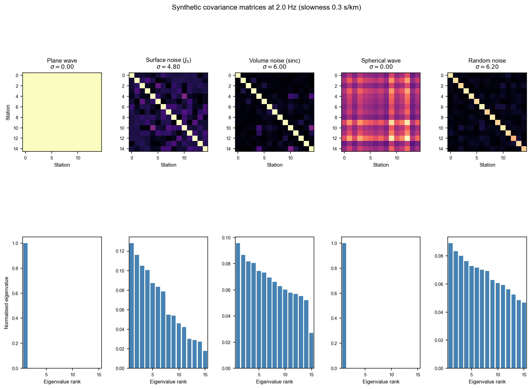
This example illustrates the different synthetic covariance matrix models provided by covseisnet.synthetic. Starting from the station geometry of the UnderVolc array at Piton de la Fournaise, we compute:

1. a plane-wave covariance — rank-1, perfectly coherent,

2. an isotropic surface-noise covariance — full-rank, described by the Bessel function \(J_0\),

3. an isotropic volume-noise covariance — full-rank, described by the sinc function,

4. a spherical-wave covariance from a point source — rank-1 with amplitude decay,

5. a random (incoherent) noise covariance — approaches the identity matrix.

For each model we display the modulus of the covariance matrix and its eigenvalue spectrum, which directly relates to the coherence of the wavefield.

import numpy as np
import matplotlib.pyplot as plt
import matplotlib.gridspec as gridspec

import covseisnet as csn
import covseisnet.synthetic as syn

Station geometry

We load the UnderVolc waveforms and their inventory so that every trace carries geographical coordinates. We then extract the list of obspy.core.trace.Stats objects — the only input required by all covseisnet.synthetic functions.

# Load waveforms and attach station coordinates
stream = csn.read("../data/undervolc.mseed")
stream.assign_coordinates("../data/undervolc.xml")

# Extract the Stats objects (one per trace)
stats = [tr.stats for tr in stream]
n_stations = len(stats)
print(f"Array: {n_stations} stations")

Array: 15 stations

Wave parameters

We choose a frequency of 2 Hz and a slowness of 0.3 s/km, which corresponds to an apparent velocity of about 3.3 km/s — a typical surface-wave velocity in volcanic settings.

frequency = 2.0  # Hz
slowness = 0.3  # s/km  (apparent velocity ≈ 3.3 km/s)

Compute synthetic covariances

We compute all five models with a single call each. For the plane-wave and spherical-wave models we additionally set the propagation direction and source position.

# 1. Plane wave arriving from the north (azimuth = 0°)
cov_plane = syn.plane_wave_covariance(stats, frequency, slowness, azimuth=0.0)

# 2. Isotropic 2-D (surface) noise
cov_surface = syn.surface_noise_covariance(stats, frequency, slowness)

# 3. Isotropic 3-D (volume) noise
cov_volume = syn.volume_noise_covariance(stats, frequency, slowness)

# 4. Spherical wave from a synthetic source 10 km south of the array centre,
#    at 5 km depth
lons = [s.coordinates["longitude"] for s in stats]
lats = [s.coordinates["latitude"] for s in stats]
source = (np.mean(lons), np.mean(lats) - 0.09, 5.0)  # ~10 km south, 5 km deep
cov_spherical = syn.spherical_wave_covariance(
    stats, frequency, slowness, source
)

# 5. Random (incoherent) noise — averaged over 500 snapshots for a smooth result
cov_noise = syn.random_noise_covariance(stats, n_snapshots=500, seed=42)

Visualize covariance matrices and eigenvalue spectra

For each model we show the normalised modulus \(|C_{ij}|/\max|C_{ij}|\) and the normalised eigenvalue distribution \(\lambda_i / \sum_j \lambda_j\). The spectral width \(\sigma\) reported in the title is the coherence measure implemented in CovarianceMatrix.coherence(kind='spectral_width').

models = [
    (cov_plane, "Plane wave"),
    (cov_surface, "Surface noise ($J_0$)"),
    (cov_volume, "Volume noise (sinc)"),
    (cov_spherical, "Spherical wave"),
    (cov_noise, "Random noise"),
]

fig = plt.figure(figsize=(14, 9))
gs = gridspec.GridSpec(2, len(models), figure=fig, hspace=0.45, wspace=0.35)

for col, (cov, label) in enumerate(models):
    # Normalised modulus
    ax_mat = fig.add_subplot(gs[0, col])
    modulus = np.abs(cov)
    ax_mat.imshow(
        modulus / modulus.max(),
        vmin=0,
        vmax=1,
        cmap="magma",
        aspect="equal",
        interpolation="nearest",
    )
    sw = float(cov.coherence(kind="spectral_width"))
    ax_mat.set_title(f"{label}\n$\\sigma={sw:.2f}$", fontsize=9)
    ax_mat.set_xlabel("Station", fontsize=8)
    if col == 0:
        ax_mat.set_ylabel("Station", fontsize=8)
    ax_mat.tick_params(labelsize=7)

    # Eigenvalue spectrum
    eigenvalues = np.linalg.eigvalsh(cov)
    eigenvalues = np.sort(eigenvalues.real)[::-1]
    eigenvalues = np.maximum(eigenvalues, 0)  # clip numerical noise
    eigenvalues /= eigenvalues.sum()  # normalise

    ax_eig = fig.add_subplot(gs[1, col])
    ax_eig.bar(
        range(1, n_stations + 1), eigenvalues, color="steelblue", width=0.8
    )
    ax_eig.set_xlabel("Eigenvalue rank", fontsize=8)
    if col == 0:
        ax_eig.set_ylabel("Normalised eigenvalue", fontsize=8)
    ax_eig.set_xlim(0.5, n_stations + 0.5)
    ax_eig.tick_params(labelsize=7)

fig.suptitle(
    f"Synthetic covariance matrices at {frequency} Hz "
    f"(slowness {slowness} s/km)",
    fontsize=11,
)
plt.show()

Interpretation

Model	Rank	Spectral width \(\sigma\)	Physical interpretation
Plane wave	1	0 (minimum)	Single coherent propagating wave
Surface noise	\(N\)	intermediate	Isotropic 2-D diffuse field
Volume noise	\(N\)	intermediate	Isotropic 3-D diffuse field
Spherical wave	1	0 (minimum)	Point source, geometrical spreading
Random noise	\(N\)	\((N-1)/2\) (maximum)	Fully incoherent field

The spectral width \(\sigma = \sum_{i=0}^{N-1} i\,\lambda_i\) (normalised eigenvalues sorted descending) ranges from 0 (rank-1, energy at index 0) to \((N-1)/2\) (uniform distribution, fully incoherent). It is monitored by CovarianceMatrix.coherence(kind="spectral_width") in real-data workflows.