Plane-wave beamforming

Frequency-domain plane-wave beamforming.

This module provides the PlaneWaveBeamforming class, which evaluates the Bartlett (conventional) beamformer power over a SlownessGrid using a CovarianceMatrix as input.

The Bartlett beamformer represents the classical steered-response-power estimator. The minimum-variance distortionless-response (MVDR/Capon) beamformer and the MUSIC pseudo-spectrum are planned for future releases.

Classes

• PlaneWaveBeamforming — Bartlett plane-wave beamformer output on a slowness grid.

class covseisnet.beamforming.PlaneWaveBeamforming(delays: PlaneWaveDelays)

Bases: SlownessGrid

Bartlett plane-wave beamforming power on a slowness grid.

Given a CovarianceMatrix \(\mathbf{C} \in \mathbb{C}^{N \times N}\) and a steering vector

\[\mathbf{a}(f, u_x, u_y) = \exp\!\bigl(-2\pi i f \boldsymbol{\tau}(u_x, u_y)\bigr)\]

where \(\boldsymbol{\tau}\) is the vector of inter-station delays from a PlaneWaveDelays object, the Bartlett beamformed power is

\[P_{\mathrm{Bartlett}}(f, u_x, u_y) = \mathbf{a}^\dagger \mathbf{C} \mathbf{a} \;\bigg/\; N^2\]

where \(N\) is the number of stations and the denominator normalises the output to the interval \([0, 1]\) for a unit-power source.

The result is stored as a 2-D array of shape (n_slowness, n_azimuth) that inherits from SlownessGrid.

Note

Planned extensions

• Temporal beamforming: applying the same steering in the time domain, which can be efficient for broadband, transient sources.

• MVDR / Capon beamformer: minimises output power subject to a distortionless constraint; suppresses correlated noise but requires matrix inversion.

• MUSIC pseudo-spectrum: projects steering vectors onto the noise subspace of the covariance matrix; provides higher resolution than Bartlett but requires knowledge of the signal subspace rank.

Parameters:

delays (PlaneWaveDelays) -- Pre-computed inter-station plane-wave delays.

Example

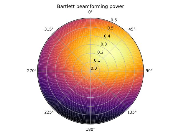
Compute the beamforming power for a synthetic plane wave:

import numpy as np
import matplotlib.pyplot as plt

import covseisnet as csn
from covseisnet.slowness import PlaneWaveDelays
from covseisnet.beamforming import PlaneWaveBeamforming
from covseisnet.synthetic import plane_wave_covariance

# Build a small circular array of 8 stations
n = 8
angles = np.linspace(0, 2 * np.pi, n, endpoint=False)
lons = 0.4 * np.cos(angles) / 111.195 + 2.0
lats = 0.4 * np.sin(angles) / 111.195 + 48.0
stats = [csn.NetworkStream.read()[0].stats.__class__() for _ in range(n)]
for i, s in enumerate(stats):
    s.coordinates = {
        "longitude": lons[i], "latitude": lats[i], "elevation": 0.0
    }

# Synthetic plane-wave covariance
frequency = 1.0
slowness  = 0.30
azimuth   = 45.0
cov = plane_wave_covariance(stats, frequency, slowness, azimuth)

# Beamforming
delays = PlaneWaveDelays(stats, slowness_max=0.6, n_slowness=60, n_azimuth=120)
bf = PlaneWaveBeamforming(delays)
bf.compute_bartlett(cov, frequency)

# Plot
S, A = delays.mesh
fig, ax = plt.subplots(subplot_kw={"projection": "polar"})
ax.pcolormesh(np.radians(A), S, bf, cmap="inferno")
ax.set_theta_direction(-1)
ax.set_theta_zero_location("N")
ax.set_title("Bartlett beamforming power")
plt.tight_layout()

Parameters:

delays (PlaneWaveDelays) -- Pre-computed inter-station plane-wave delays.

compute_bartlett(covariance: CovarianceMatrix, frequency: float) → None

Compute the Bartlett beamforming power in-place.

Evaluates

\[P(u_x, u_y) = \mathbf{a}^\dagger(f,u_x,u_y)\, \mathbf{C}\, \mathbf{a}(f,u_x,u_y) \;/\; N^2\]

for every grid point and stores the result in the array.

Parameters:

• covariance (CovarianceMatrix) -- The spectral covariance matrix at one time–frequency bin, of shape (n_stations, n_stations).

• frequency (float) -- The frequency in Hz at which to evaluate the steering vectors.

Raises:

ValueError -- If covariance does not have exactly 2 dimensions.