Locating an earthquake with matched-field processing

Matched-field processing (MFP) extends plane-wave beamforming to three dimensions by replacing the plane-wave steering vector with a replica — a predicted wavefield for a point source at each candidate grid location. This allows simultaneous estimation of back-azimuth, horizontal range, and depth.

This example locates the Mb 4.4 earthquake that occurred in the Aegean Sea on 5 October 2020 (39.88°N, 23.35°E, 10 km depth), using the same regional network as the back-projection example. We demonstrate:

1. Building a constant-velocity model over the network area,

2. Computing per-station travel-time grids with covseisnet.travel_times.TravelTimes,

3. Validating the Bartlett and MVDR processors on a synthetic covariance injected at the known epicentre,

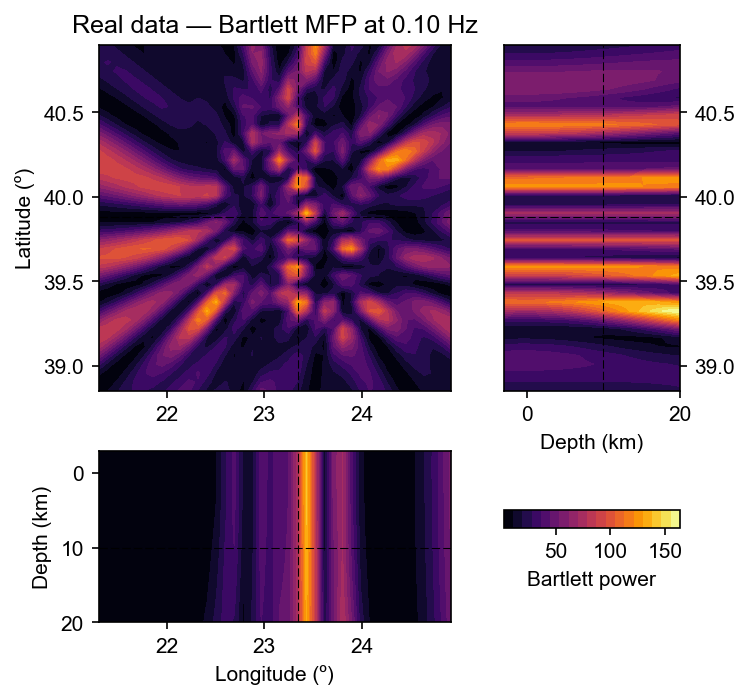
4. Applying the processors to the real earthquake covariance and comparing the recovered location with the catalogue position.

from cartopy.crs import PlateCarree
import numpy as np
import matplotlib.pyplot as plt

import covseisnet as csn
from covseisnet.matchedfield import MatchedFieldProcessing
import covseisnet.synthetic as syn

Load seismograms and station coordinates

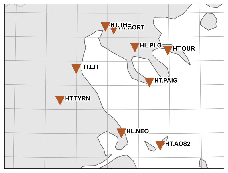
We load the Aegean Sea example data, download the station inventory from the National Observatory of Athens (NOA), and pre-process the waveforms exactly as in the back-projection example: merge, detrend, high-pass filter, and synchronise. We also plot the station map with the known catalogue epicentre, and capture the map extent for use in the velocity model grid.

# Load seismograms
stream = csn.NetworkStream.read("../data/aegean_sea_example.mseed")

# Pre-process
stream.merge(1, fill_value=0)
stream.detrend("linear")
stream.filter("highpass", freq=0.01)
stream.synchronize()

# Download inventory and attach coordinates
inventory = stream.download_inventory(datacenter="NOA")
stream.assign_coordinates(inventory)

stats = [tr.stats for tr in stream]
n_stations = len(stats)
lons = np.array([s.coordinates["longitude"] for s in stats])
lats = np.array([s.coordinates["latitude"] for s in stats])
print(f"Array: {n_stations} stations")

# Known catalogue location (lon, lat, depth_km)
source_location = (23.3465, 39.8812, 10.0)

# Station map with catalogue epicentre
fig = inventory.plot(projection="local", resolution="h")
fig.axes[0].plot(
    *source_location[:2],
    "k*",
    markersize=20,
    transform=PlateCarree(),
    label="Catalogue",
)

# Natural extent of the map (reused for the velocity-model grid)
extent = fig.axes[0].get_extent(crs=PlateCarree())

Array: 9 stations

Velocity model and travel times

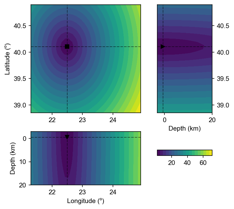
We build a constant-velocity model at 3.5 km/s (S-wave dominated) over the geographic extent returned by the station map, extended from −3 to 20 km depth to encompass both shallow and crustal sources. For each station we compute the travel time from every grid point to that receiver.

# Append depth range to the horizontal extent from the map
extent_with_depth = extent + (-3, 20)

velocity_model = csn.velocity.VelocityModel(
    extent=extent_with_depth, shape=(30, 30, 20), velocity=3.5
)

# Per-station travel-time grids
travel_times = {
    tr.stats.station: csn.calculate_travel_times(
        velocity_model, stats=tr.stats
    )
    for tr in stream
}
print(f"TravelTimes grid shape: {next(iter(travel_times.values())).shape}")

# Station coordinates for plotting
receiver_coords = None

TravelTimes grid shape: (30, 30, 20)

csn.plot.grid3d(
    travel_times["LIT"],
    # receiver_coords=receiver_coords,
    # source_location=source_location,
)

(<Figure size 750x750 with 4 Axes>,
 {'xy': <Axes: label='xy', ylabel='Latitude (º)'>,
  'zy': <Axes: label='zy', xlabel='Depth (km)'>,
  'xz': <Axes: label='xz', xlabel='Longitude (º)', ylabel='Depth (km)'>,
  'cb': <Axes: label='cb'>})

(travel_times["LIT"].lon[1] - travel_times["LIT"].lon[0]) * 111

np.float64(6.782131466347639)

Validation on a synthetic spherical wave

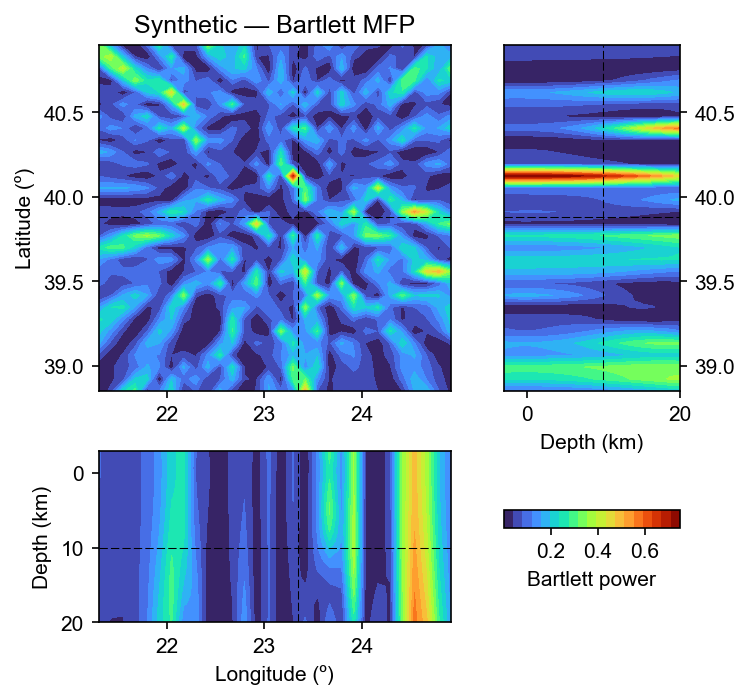
Before applying MFP to the real earthquake we verify the implementation by injecting a synthetic rank-1 covariance at the catalogue epicentre (23.35°E, 39.88°N, 10 km depth) and checking that the Bartlett processor recovers that location.

source = source_location
frequency = 0.2  # Hz — wavelength ~70 km, well above grid spacing (~12 km)
slowness = 1 / 3.5  # s/km — matching the velocity model

cov_synth = syn.spherical_wave_covariance(stats, frequency, slowness, source)
cov_synth /= np.abs(cov_synth)

mfp = MatchedFieldProcessing(travel_times)
mfp.compute_bartlett(cov_synth, frequency)

lon_det, lat_det, dep_det = mfp.maximum_coordinates()
print(
    f"True source  : lon={source[0]:.3f}° lat={source[1]:.3f}° depth={source[2]:.1f} km"
)
print(
    f"MFP estimate : lon={lon_det:.3f}° lat={lat_det:.3f}° depth={dep_det:.1f} km"
)

True source  : lon=23.346° lat=39.881° depth=10.0 km
MFP estimate : lon=23.292° lat=40.124° depth=-0.6 km

fig, ax = csn.plot.grid3d(
    mfp,
    profile_coordinates=source,
    cmap="turbo",
    label="Bartlett power",
)
ax["xy"].set_title("Synthetic — Bartlett MFP")

Text(0.5, 1.0, 'Synthetic — Bartlett MFP')

MVDR matched-field processor

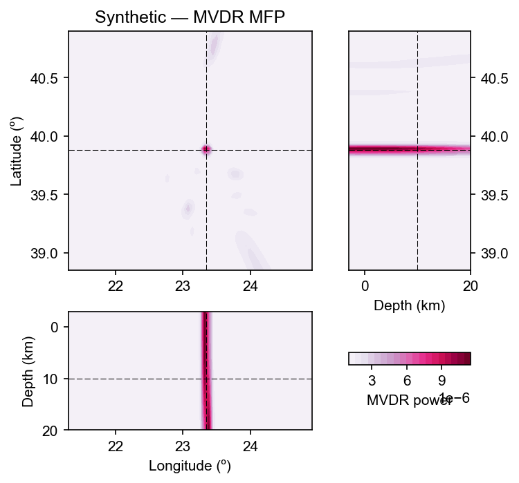
The MVDR (minimum-variance distortionless-response) processor typically achieves higher spatial resolution than Bartlett by suppressing the sidelobe structure at the cost of a matrix inversion. We apply it to the same synthetic covariance and compare the horizontal slice with the Bartlett result.

mfp_mvdr = MatchedFieldProcessing(travel_times)
mfp_mvdr.compute_mvdr(cov_synth, frequency)

lon_mv, lat_mv, dep_mv = mfp_mvdr.maximum_coordinates()
print(
    f"MVDR estimate: lon={lon_mv:.3f}° lat={lat_mv:.3f}° depth={dep_mv:.1f} km"
)

fig, ax = csn.plot.grid3d(
    mfp_mvdr,
    profile_coordinates=source,
    cmap="PuRd",
    label="MVDR power",
)
ax["xy"].set_title("Synthetic — MVDR MFP")

MVDR estimate: lon=23.320° lat=39.894° depth=0.5 km

Text(0.5, 1.0, 'Synthetic — MVDR MFP')

Application to the real earthquake recording

Two constraints set the usable frequency band:

1. Spatial sampling: the Bartlett steering vector \(e^{-2\pi i f \tau}\) oscillates at wavelength \(\lambda = v/f\). Correct resolution requires at least two grid points per wavelength. With a horizontal grid spacing of ~15–20 km, frequencies above ~0.1 Hz are aliased and the power maximum lands at an arbitrary grid point.

2. Incoherent stacking: at a single frequency the Bartlett map contains grating lobes. Averaging the power incoherently over a frequency band suppresses them because the lobes shift with frequency while the true source maximum stays fixed.

We therefore filter the data to 0.02–0.1 Hz (surface-wave dominated), use a 300 s window to capture all regional arrivals, and stack the Bartlett power over the band.

# Work on a copy so accumulated filters don't contaminate the stream
stream_lf = stream.copy()
stream_lf.filter("bandpass", freqmin=0.02, freqmax=0.1)

# 300 s window captures all regional surface-wave arrivals
times, frequencies, covariances = csn.calculate_covariance_matrix(
    stream_lf, window_duration=300, average=1, whiten="none"
)

# Frequency band for incoherent stacking
fmin, fmax = 0.02, 0.1
freq_mask = (frequencies >= fmin) & (frequencies <= fmax)
print(f"Stacking {freq_mask.sum()} frequency bins ({fmin}–{fmax} Hz)")

Using frequency 0.100 Hz

# Incoherent frequency stacking over the 0.02–0.1 Hz band
power_stack = np.zeros(next(iter(travel_times.values())).shape)
for f, cov_f in zip(frequencies[freq_mask], covariances[0, freq_mask]):
    mfp_f = MatchedFieldProcessing(travel_times)
    mfp_f.compute_bartlett(cov_f, f)
    power_stack += np.nan_to_num(mfp_f)
power_stack /= freq_mask.sum()

# Store in a MatchedFieldProcessing object so grid3d can plot it
mfp_real = MatchedFieldProcessing(travel_times)
mfp_real[...] = power_stack

lon_r, lat_r, dep_r = mfp_real.maximum_coordinates()
print(f"MFP estimate : lon={lon_r:.3f}° lat={lat_r:.3f}° depth={dep_r:.1f} km")
print(
    f"Catalogue    : lon={source[0]:.3f}° lat={source[1]:.3f}° depth={source[2]:.1f} km"
)

fig, ax = csn.plot.grid3d(
    mfp_real,
    profile_coordinates=source_location,
    cmap="inferno",
    label="Bartlett power (0.02–0.1 Hz stack)",
)
ax["xy"].set_title(f"Real data — Bartlett MFP ({fmin}–{fmax} Hz)")

MFP estimate : lon=23.337° lat=39.324° depth=20.0 km
Catalogue    : lon=23.346° lat=39.881° depth=10.0 km

Text(0.5, 1.0, 'Real data — Bartlett MFP at 0.10 Hz')