Plane-wave beamforming

This example demonstrates frequency-domain plane-wave beamforming with the covseisnet.beamforming module. Starting from the UnderVolc array at Piton de la Fournaise, we:

1. Pre-process the seismograms and estimate the spectral covariance matrix,

2. Build a slowness grid and pre-compute the inter-station plane-wave delays with covseisnet.slowness.PlaneWaveDelays,

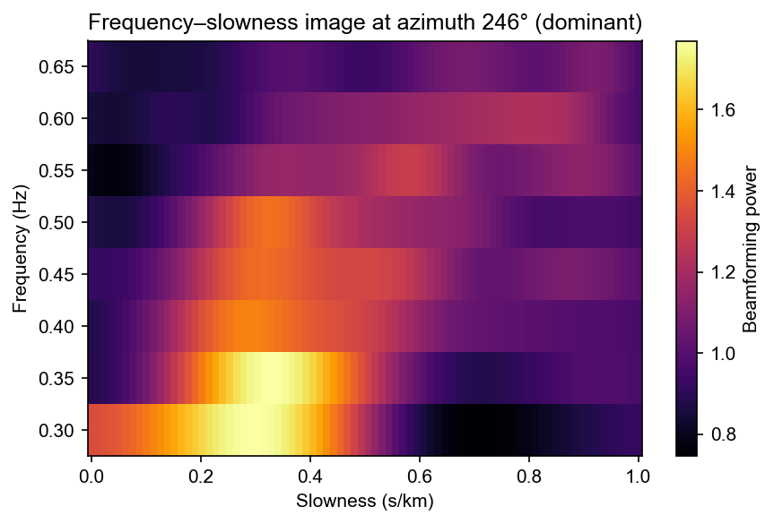
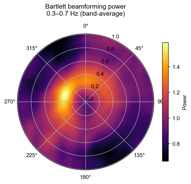
3. Apply the Bartlett (conventional) beamformer with covseisnet.beamforming.PlaneWaveBeamforming.compute_bartlett,

4. Display the beamforming power as a polar diagram and as a frequency–slowness image.

We first validate the method on a synthetic plane-wave covariance, then apply it to the real seismograms.

import numpy as np
import matplotlib.pyplot as plt

import covseisnet as csn
from covseisnet.slowness import PlaneWaveDelays
from covseisnet.beamforming import PlaneWaveBeamforming
import covseisnet.synthetic as syn

Station geometry

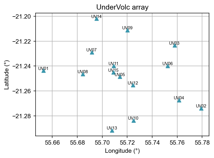
We load the UnderVolc seismograms and attach geographical coordinates. Only the first 200 seconds of data are used to keep the example fast.

# Load waveforms and attach station coordinates
stream = csn.read("../data/undervolc.mseed")
stream.assign_coordinates("../data/undervolc.xml")

# Extract stats list
stats = [tr.stats for tr in stream]
n_stations = len(stats)
print(f"Array: {n_stations} stations")

# Quick station map
lons = [s.coordinates["longitude"] for s in stats]
lats = [s.coordinates["latitude"] for s in stats]
fig, ax = plt.subplots(figsize=(5, 4))
ax.scatter(lons, lats, marker="^", zorder=3)
for s in stats:
    ax.annotate(
        s.station,
        (s.coordinates["longitude"], s.coordinates["latitude"]),
        fontsize=7,
        ha="center",
        va="bottom",
    )
ax.set_xlabel("Longitude (°)")
ax.set_ylabel("Latitude (°)")
ax.set_title("UnderVolc array")
ax.set_aspect("equal")
ax.grid()
plt.tight_layout()

Array: 15 stations

Validation on a synthetic plane wave

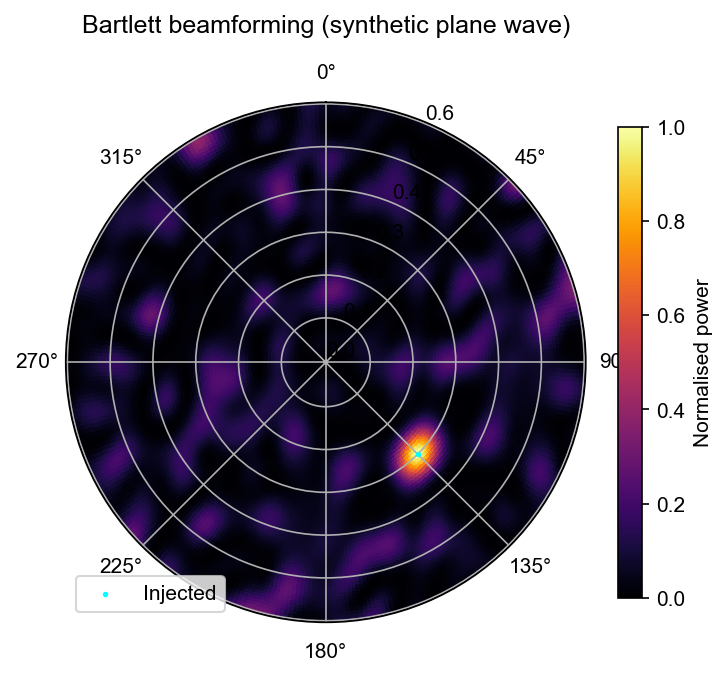
Before applying beamforming to real data we verify that the method correctly recovers the injected slowness and azimuth using a synthetic rank-1 covariance from covseisnet.synthetic.plane_wave_covariance.

# Parameters
frequency = 1.0  # Hz
slowness = 0.30  # s/km  (~3.3 km/s)
azimuth = 135.0  # degrees clockwise from North (SE)

# Synthetic rank-1 covariance
cov_plane = syn.plane_wave_covariance(stats, frequency, slowness, azimuth)
cov_plane /= np.abs(cov_plane)

# Slowness grid
delays = PlaneWaveDelays(stats, slowness_max=0.6, n_slowness=80, n_azimuth=360)

# Beamforming
bf = PlaneWaveBeamforming(delays)
bf.compute_bartlett(cov_plane, frequency)

s_det, az_det = bf.maximum_coordinates()
print(f"Injected : slowness = {slowness:.3f} s/km, azimuth = {azimuth:.1f}°")
print(f"Detected : slowness = {s_det:.3f} s/km, azimuth = {az_det:.1f}°")

# Polar plot
S, A = delays.mesh
fig, ax = plt.subplots(subplot_kw={"projection": "polar"}, figsize=(5, 5))
pcm = ax.pcolormesh(
    np.radians(A),
    S,
    bf,
    cmap="inferno",
    shading="auto",
    vmin=0,
    vmax=1,
)
ax.scatter(
    np.radians(azimuth),
    slowness,
    marker=".",
    s=10,
    color="cyan",
    zorder=5,
    label="Injected",
)
ax.set_theta_direction(-1)
ax.set_theta_zero_location("N")
ax.set_title("Bartlett beamforming (synthetic plane wave)", pad=15)
plt.colorbar(pcm, ax=ax, label="Normalised power", shrink=0.7)
ax.legend(loc="lower left")
plt.tight_layout()

Injected : slowness = 0.300 s/km, azimuth = 135.0°
Detected : slowness = 0.296 s/km, azimuth = 135.0°

Spectral covariance from real data

We estimate the spectral covariance matrix by windowing the data into overlapping segments of 20 s, applying spectral whitening, and averaging over all windows. This yields a single covariance matrix as a function of frequency, representative of the ambient noise field recorded by the array.

# Normalise and filter before covariance estimation
stream.detrend("linear")
stream.filter("bandpass", freqmin=0.5, freqmax=10.0)

# Covariance matrix
times, frequencies, covariances = csn.calculate_covariance_matrix(
    stream, window_duration=20, average=10, whiten="slice"
)

# Average over time to get a single N×N matrix per frequency
cov_mean = covariances.mean(axis=0)
print(f"Covariance shape: {cov_mean.shape}  (n_freq × N × N)")

/Users/seydoux/GitHub/covseisnet/.venv/lib/python3.13/site-packages/obspy/signal/filter.py:62: UserWarning: Selected high corner frequency (10.0) of bandpass is at or above Nyquist (10.0). Applying a high-pass instead.
  warnings.warn(msg)

Covariance shape: (201, 15, 15)  (n_freq × N × N)

Beamforming power as a function of frequency

We apply the Bartlett beamformer at every frequency bin and accumulate the result into a frequency–slowness–azimuth cube. We then visualise:

• The polar diagram (azimuth × slowness) integrated over a 1–4 Hz band, showing the dominant propagation direction of the ambient wavefield.

• The frequency–slowness image at the dominant azimuth.

# Reuse the same delay grid
delays = PlaneWaveDelays(stats, slowness_max=1, n_slowness=80, n_azimuth=360)

# Frequency band for integration
fmin, fmax = 0.3, 0.7
freq_mask = (frequencies >= fmin) & (frequencies <= fmax)

# Accumulate beamforming power over the chosen frequency band
bf_stack = np.zeros(delays.shape)
n_freq = 0
for f, cov_f in zip(frequencies[freq_mask], cov_mean[freq_mask]):
    bf = PlaneWaveBeamforming(delays)
    bf.compute_bartlett(cov_f, f)
    bf_stack += np.nan_to_num(bf)
    n_freq += 1
bf_stack /= n_freq

# ---- Polar diagram (band-integrated) ----
S, A = delays.mesh
fig, ax = plt.subplots(subplot_kw={"projection": "polar"}, figsize=(5, 5))
pcm = ax.pcolormesh(
    np.radians(A),
    S,
    bf_stack,
    cmap="inferno",
    shading="auto",
)
ax.set_theta_direction(-1)
ax.set_theta_zero_location("N")
ax.set_title(
    f"Bartlett beamforming power\n{fmin}–{fmax} Hz (band-average)", pad=15
)
plt.colorbar(pcm, ax=ax, label="Power", shrink=0.7)
plt.tight_layout()

# ---- Frequency–slowness image at the dominant azimuth ----
i_az_max = np.argmax(bf_stack.sum(axis=0))
az_dominant = delays.azimuth[i_az_max]

# Build the frequency–slowness matrix
fs_image = np.zeros((freq_mask.sum(), len(delays.slowness)))
for i_f, (f, cov_f) in enumerate(
    zip(frequencies[freq_mask], cov_mean[freq_mask])
):
    bf_f = PlaneWaveBeamforming(delays)
    bf_f.compute_bartlett(cov_f, f)
    fs_image[i_f] = bf_f[:, i_az_max]

fig, ax = plt.subplots(figsize=(6, 4))
pcm = ax.pcolormesh(
    delays.slowness,
    frequencies[freq_mask],
    fs_image,
    cmap="inferno",
    shading="auto",
)
ax.set_xlabel("Slowness (s/km)")
ax.set_ylabel("Frequency (Hz)")
ax.set_title(
    f"Frequency–slowness image at azimuth {az_dominant:.0f}° (dominant)"
)
plt.colorbar(pcm, ax=ax, label="Beamforming power")
plt.tight_layout()